Insights
Ultrasound Attenuation Estimation: Keep System Response Out of the Slope
Separate sample attenuation from acquisition-chain changes with matched reference-phantom spectra, an exact gain-mismatch example and a proposed ultrasound OEM verification procedure.
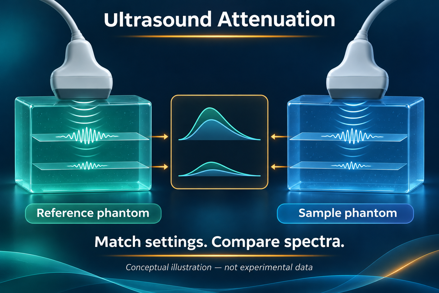
Conceptual illustration — not experimental data. The paired views represent sequential acquisitions with the same probe.
Engineering question: When an ultrasound attenuation estimate changes, how can an OEM team determine whether the change came from the sample or from the acquisition chain?
A useful verification target is an attenuation estimate that remains stable when a permitted system setting changes and the matching reference acquisition is updated. This article develops a proposed engineering test around that target. It does not report ALEVA device measurements or clinical diagnostic performance.
What a reference phantom can remove
In the reference phantom method, echo spectra from the sample are compared with spectra from a phantom whose acoustic properties are known. The foundational work by Yao, Zagzebski and Madsen used this comparison to account for depth-dependent instrumentation factors. The reference is part of the measurement procedure, not simply a phantom image kept in a folder. Yao et al., 1990.
For an OEM implementation, pair the reference and sample records by probe identity, transmit waveform, receive configuration, focus, aperture, time-gain compensation, sampling and reconstruction settings. Define the RF or linear-IQ output boundary and its scaling. A display screenshot is not a substitute for a documented spectral input. These are proposed interface requirements, not evidence that any particular commercial system exposes those controls.
Define the coefficient before fitting the slope
Consider an ideal homogeneous sample and reference with matched propagation geometry and system response. Let Pₛ(f,z) and Pᵣ(f,z) be their averaged echo power spectra, and define R(f,z) = 10 log₁₀[Pₛ(f,z)/Pᵣ(f,z)]. If the one-way attenuation coefficients aₛ and aᵣ are expressed in dB/cm at frequency f, the pulse-echo model gives:
R(f,z) = C(f) − 2[aₛ(f) − aᵣ(f)]z.
C(f) absorbs the depth-independent backscatter ratio. The factor two represents the outgoing and returning paths. Thus, aₛ(f) = aᵣ(f) − ½ ∂R/∂z. This is the decibel form of the reference-phantom power-ratio model; coefficients expressed in nepers require a different numerical factor. The assumptions include locally uniform scattering statistics, negligible additive noise and clutter, and adequately matched diffraction. Yao et al., 1991.
A reproducible gain-mismatch example
The following is an exact educational calculation, not simulated tissue data or a measured device result. Assume attenuation is linear with frequency over the selected band. Set the reference slope to 0.50 dB/cm/MHz and the sample slope to 0.70 dB/cm/MHz. At 5 MHz, over a 2 cm depth interval, the ideal change in R is −2 × (0.70 − 0.50) × 5 × 2 = −4 dB. Substitution into the estimator returns 0.70 dB/cm/MHz.
Now introduce a sample-only gain mismatch that adds 2 dB to R across that same depth interval. The observed change becomes −2 dB, and the inferred attenuation slope becomes 0.50 − (−2)/(2 × 5 × 2) = 0.60 dB/cm/MHz. The material has not changed. A constant gain offset would change the intercept in this ideal model; a depth-dependent mismatch changes the slope. This distinction is a useful software test fixture, but it does not bound the error of a real scanner.
Challenge the cancellation assumptions
A 2025 peer-reviewed phantom study by Whitson, Rosado-Mendez and Hall compared conventional spectral-difference attenuation estimation with regularized ALGEBRA estimates under deliberately introduced acoustic clutter. It found advantages for the regularized methods in the tested conditions, with variance reduction contributing substantially to the improvement. That result supports testing clutter explicitly; it does not establish that regularization eliminates model error in arbitrary probes or acquisition modes. Whitson et al., 2025.
For the proposed OEM test, retain both the fitted slope and its residuals. Evaluate repeat captures, changes in the usable frequency band, and depth intervals that approach the noise floor. Add a separately documented clutter condition. A smoother parameter map should not pass merely because its visual variability is lower: compare bias against a characterized target as well as repeatability.
Longer depth intervals provide more leverage for slope estimation, while smaller regions preserve spatial locality. Increasing overlap between spectral windows does not automatically create independent measurements. The uncertainty analysis of Yao and colleagues makes independent information and the estimation depth range explicit. Select region size and averaging together, and record the resulting spatial averaging rather than reporting the output pixel size as the parameter-map resolution. Yao et al., 1991.
Separate the validation tests
Arithmetic test: verify the coefficient units, round-trip factor, sign and recovery of the two educational cases above.
Paired-acquisition test: repeat the same characterized target under declared operating settings, acquiring a matching reference for each configuration. Retain rejected regions and reasons.
Mismatch test: intentionally replay an incompatible reference configuration. Verify that metadata checks reject it or that the output is explicitly marked outside the validated conditions.
Robustness test: introduce documented clutter, reduced signal level and region heterogeneity separately. Report bias, repeatability, valid-region coverage and processing time together.
Set acceptance limits from the intended engineering use and measured uncertainty before selecting an algorithm. A low average error does not compensate for silent failures in part of the declared operating range.
The OEM decision
A reference phantom is not the only route. Gong and colleagues reported a reference-frequency method in 2019 that normalizes neighboring frequency components without a separate reference phantom. It is an alternative estimation model, not a general exemption from acquisition and validation requirements. Gong et al., 2019.
For an ultrasound OEM development scope, make the handover include acquisition metadata, reference characterization, estimator version, valid frequency and depth ranges, uncertainty evidence and failure reporting. The deliverable should be a reproducible measurement procedure, not only an attenuation number.
Image note: AI-generated conceptual illustration, not experimental data or ALEVA hardware. The two illustrated probes represent paired acquisitions; the procedure described here uses the same probe and matched settings sequentially. The stylized spectra are not the numerical example above.
Author: ALEVA · Orange County, California, USA.
Sources and publication dates
Yao LX, Zagzebski JA, Madsen EL. Backscatter Coefficient Measurements Using a Reference Phantom to Extract Depth-Dependent Instrumentation Factors. Ultrasonic Imaging 12(1), 58–70, January 1990. Peer-reviewed. DOI: 10.1177/016173469001200105.
Yao LX, Zagzebski JA, Madsen EL. Statistical uncertainty in ultrasonic backscatter and attenuation coefficients determined with a reference phantom. Ultrasound in Medicine & Biology 17(2), 187–194, 1991. Peer-reviewed. DOI: 10.1016/0301-5629(91)90126-H; public university-hosted manuscript.
Whitson HM, Rosado-Mendez IM, Hall TJ. Clutter-Generating Phantom Material. Part II: Utilization in the Comparison of Conventional and Regularized Ultrasound Attenuation Estimation. Ultrasound in Medicine & Biology 51(5), 777–787, May 2025; published online February 11, 2025. Peer-reviewed, publicly available author manuscript. DOI: 10.1016/j.ultrasmedbio.2025.01.006; full text.
Gong P, Song P, Huang C, Trzasko J, Chen S. System-Independent Ultrasound Attenuation Coefficient Estimation Using Spectra Normalization. IEEE Transactions on Ultrasonics, Ferroelectrics, and Frequency Control 66(5), 867–875, May 2019; published online March 5, 2019. Peer-reviewed. DOI: 10.1109/TUFFC.2019.2903010.