Insights
Ultrasound Speckle Tracking: Validate the Motion and the Confidence
A source-led OEM verification framework for ultrasound displacement tracking, with an exact analytical example separating correlation scores from evidence of motion accuracy.
ALEVA · Orange County, California, USA
Engineering question: When an ultrasound motion tracker reports a plausible displacement and a high correlation score, what evidence makes that estimate trustworthy?
For an OEM team, the useful deliverable is a displacement estimate accompanied by evidence about when it becomes unreliable. A smooth motion field can be visually convincing while concealing rejected measurements, excessive regularization or a mismatch between the acquisition and the estimator. The acceptance test should expose those conditions before downstream software treats every vector as valid.
Specify what the tracker actually sees
Tracking may operate on RF samples, complex IQ data or envelope/B-mode images. These are different inputs with different information and processing histories. The 2024 review by Ashikuzzaman and colleagues surveys correlation, model-based, energy-based and learning-based approaches, including challenges in lateral and large-displacement estimation. It provides a useful framework for choosing an estimator, rather than a universal recommendation for one algorithm. [1]
Our proposed integration record starts with the signal domain, spatial sampling, frame timestamps, beamforming preset and all processing applied before tracking. Record the matching-window dimensions in physical units as well as samples, the permitted search range, interpolation method and boundary handling. A parameter named “window size” is insufficient when different probes or export paths produce different pixel spacing.
Separate displacement from frame-pair quality
Caius and colleagues, in a peer-reviewed study published on 3 June 2026, assessed RF frame-pair quality by comparing the measured post-compression frame with a version of the pre-compression frame warped using the estimated displacement. They evaluated correlation and mean squared error, with controlled out-of-plane corruption and experimental data. This supports evaluating the consistency of an estimated motion field with its input data. It does not make their numerical thresholds universal across scanners, preprocessing pipelines or applications. [2]
For an OEM acceptance test, we recommend recording both the estimated displacement and the quality evidence used to retain or reject it. Where independent reference motion is available, compare the quality score against actual displacement error. A score calculated from the same images used to fit the motion is an internal consistency measure; it is not independent ground truth.
An exact example: the same score, different causes
Consider a deliberately simplified, one-dimensional model. Let f(x) and h(x) be independent, zero-mean stationary signals with unit variance. Let f have autocorrelation R(r) = exp[−r²/(2ℓ²)], where ℓ is a correlation length. Define a second signal as g(x) = c f(x−d) + √(1−c²) h(x) + n(x). Here d is the true translation, c ranges from zero to one and represents retained signal correlation, and n is independent zero-mean noise with variance η². The reference f is noise-free.
At residual alignment error r, the population normalized correlation is:
ρ(r) = c exp[−r²/(2ℓ²)] / √(1+η²).
This follows because the cross-covariance is cR(r), while the second signal has variance 1+η². At correct alignment, c = 0.8 with no added noise gives ρ = 0.8. So does c = 1 with noise RMS η = 0.75, because 1/√(1+0.75²) = 0.8. In this model, even the complete population correlation curves coincide.
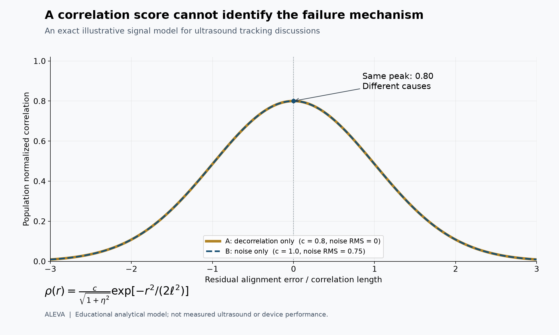
Figure: Two distinct combinations of signal decorrelation and added noise produce the same correlation curve. Original analytical illustration, not measured ultrasound, an ALEVA hardware result or a prediction of displacement accuracy.
The example shows why correlation alone cannot identify the cause of a quality loss. It does not show that the two cases have identical finite-window tracking errors. Real RF oscillations, anisotropic resolution, deformation within a window, correlated clutter, noise in both frames and out-of-plane motion are outside this model. A finite-window maximum is also a noisy statistic, unlike the population curve plotted here.
Validate preprocessing together with tracking
Xu and colleagues’ peer-reviewed 2025 study evaluated near-field clutter filtering before cross-correlation-based speckle tracking using simulated and in vivo acquisitions. Its relevance to engineering verification is that preprocessing and motion estimation were assessed together. An image-quality improvement should therefore trigger a tracking check on the resulting data, rather than serve as a substitute for one. [3]
A proposed verification sequence begins with known rigid translations, including fractional-sample shifts and motion near the search boundary. It then introduces deformation, independently varied noise and controlled decorrelation. Follow these algorithm checks with physical phantom acquisitions that include probe movement and the actual processing path. Digital shifts verify software behavior under specified assumptions; they do not reproduce every acquisition effect.
For each condition, report axial and lateral error separately, signed bias, an explicitly defined error percentile, the fraction of estimates rejected and latency on the intended hardware. Retain failed cases. Otherwise, an apparently improved error statistic may simply reflect the removal of the most difficult measurements.
Make the trade-off reviewable
Window support, search range, interpolation and regularization should be evaluated as separate design choices. Our proposed review asks whether a larger window improves robustness at the expense of resolving local motion variation, whether stronger smoothing suppresses a real displacement boundary, and whether a wider search increases ambiguous matches or compute cost. Increasing output-grid density alone is not evidence that these trade-offs have improved.
For custom probe development, include the intended probe geometry, imaging depth and acquisition preset in the verification matrix. The probe and beamformer determine the data supplied to the estimator; a tracking benchmark from a different acquisition chain is supporting evidence, not acceptance of the new chain.
The OEM handover should include a reproducible dataset, reference-motion provenance, algorithm and preprocessing versions, quality flags, explicit rejection behavior and measured execution cost. This turns a convincing demonstration into an engineering decision that another team can repeat. The workflow proposed here is an evaluation framework, not a claim that ALEVA uses a particular tracking algorithm or has validated a clinical application.
References
Ashikuzzaman M. et al. Displacement Tracking Techniques in Ultrasound Elastography: From Cross Correlation to Deep Learning. IEEE Transactions on Ultrasonics, Ferroelectrics, and Frequency Control, 71(7), 842–871, July 2024. Peer-reviewed review. DOI: 10.1109/TUFFC.2024.3410671.
Caius M., Wang Z., Czarnota G., Samani A. Data Quality Analyzer—Towards Optimal Radio-Frequency Frame Pair Selection for Ultrasound Elastography. Bioengineering, 13(6), 656, 3 June 2026. Peer-reviewed research. DOI: 10.3390/bioengineering13060656.
Xu Y., Yiu K.-H., Lee W.-N. Near-Field Clutter Mitigation in Speckle Tracking Echocardiography. Ultrasound in Medicine & Biology, 51(4), 683–694, April 2025; published online 17 January 2025. Peer-reviewed research. DOI: 10.1016/j.ultrasmedbio.2024.12.016.