Insights
Ultrasound Doppler Angle Correction: Propagate the Angle Uncertainty
How ultrasound OEM teams can propagate Doppler angle uncertainty into velocity error, separate geometric and spectral limitations, and define reproducible acceptance tests.
Engineering question: How should an ultrasound OEM validate an angle-corrected Doppler velocity when the angle itself is uncertain?
A velocity display can be numerically precise while its geometric assumption is weak. The engineering task is to preserve the measured Doppler component, state how the flow direction was obtained, and test how angular uncertainty propagates into the reported speed. This article proposes a verification procedure; it does not establish a clinical operating limit or claim measured ALEVA product performance.
Define what the correction estimates
For an ideal monostatic pulse-echo measurement with a single flow direction, the Doppler relation is fD = 2f0v cos(theta)/c. Here theta is the angle between the beam and the actual velocity vector, not automatically the angle of a visible vessel wall. Assume the sound speed c and transmitted frequency f0 used by the calculation are correct, and define the measured axial component u = cfD/(2f0).
If the software uses an estimated angle theta-hat, the reported speed is v-hat = u/cos(theta-hat). With otherwise exact data, v-hat/v = cos(theta)/cos(theta-hat). An angle cursor therefore introduces a model input; it does not provide an independent measurement of the complete velocity vector.
A reproducible sensitivity calculation
Let delta = theta-hat minus theta. The exact relative speed error is cos(theta)/cos(theta + delta) minus 1. The first-order approximation is tan(theta) multiplied by delta, with delta expressed in radians. This approximation is useful for small perturbations, but the exact expression should be used near large angles or when the error interval is not small.
For an illustrative true angle of 60 degrees, entering 65 degrees produces a +18.3% speed error; entering 55 degrees produces a -12.8% error. At a true angle of 30 degrees, the same two perturbations produce approximately +5.7% and -4.4%. These are deterministic calculations, not experimental results or acceptable clinical tolerances. The asymmetric errors also show why a symmetric angular error bar need not produce a symmetric speed interval.
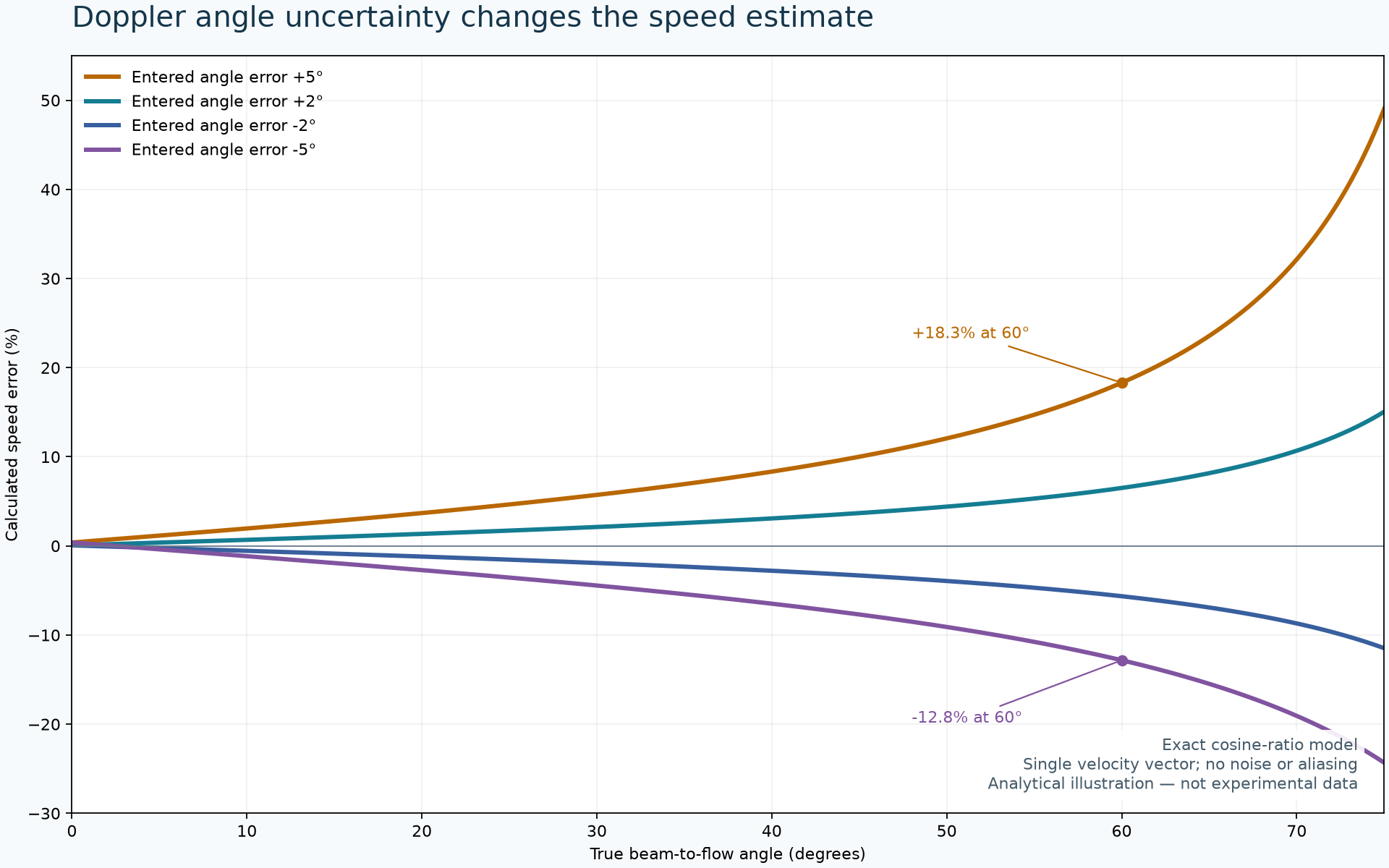
The accompanying plot evaluates the exact expression for true angles from 0 to 75 degrees and errors of plus or minus 2 and 5 degrees. It assumes one velocity vector, perfect Doppler-frequency estimation, no aliasing, and correct sound speed. It omits finite-aperture effects, clutter, noise, refraction and motion. At a perpendicular beam-flow geometry, a zero ideal Doppler component cannot establish that the material is stationary.
Keep three error mechanisms separate
Angle-estimation error: Compare the entered or automated angle against an independent geometric reference. A mean absolute angle error alone can hide a small number of large errors in especially sensitive angular ranges.
Spectral-estimation error: A correct angle does not guarantee a correct peak velocity. Miyamoto and colleagues reported peak-velocity overestimation in a 2012 string-phantom experiment even at incident angles of 60 degrees or less. That result is evidence about their experimental configuration, not a universal correction factor for another probe or estimator. [1]
Model mismatch: A two-dimensional vessel-axis estimate may not represent an out-of-plane or locally changing velocity direction. For OEM acceptance, specify whether the output is an axial component, an angle-corrected scalar, or a reconstructed vector, and how unavailable or invalid estimates are represented.
Automation and vector estimation need different validation
Patil and Anand's automated angle-estimation study is an IEEE EMBC 2019 publication. Its arXiv record was uploaded in 2025 and revised in 2026; those repository dates should not be presented as the original research date. The study compared automated angles with a human observer. Agreement with an observer is useful evidence, but it is not independent proof of physical flow direction or of the downstream velocity error in a new system. [2]
A 2026 two-beam estimation paper by Kavitha and Tiwari examines how noise, frequency uncertainty and beam geometry affect magnitude and direction estimates. The publisher identifies the available article as peer-reviewed accepted research awaiting its final Version of Record. Its theoretical and simulation results motivate geometry-aware testing; they do not validate a particular commercial implementation. [3]
For two ideal in-plane measurements, write u = A v + noise, with each row of A containing the relevant beam-direction components. Nearly parallel directions make the missing component difficult to estimate: a small measurement perturbation can cause a large reconstructed-vector change. Wider angular separation may improve this algebraic conditioning, but the usable aperture, signal quality and common sampled region must still be verified. More beams are not automatically independent information.
A proposed OEM acceptance procedure
Separate arithmetic from acquisition. Inject known Doppler shifts and angle metadata into the processing interface. Verify units, sign convention, degree-to-radian conversion and the exact cosine ratio. Include invalid and near-perpendicular inputs; require an explicit invalid state rather than a plausible-looking finite speed.
Challenge geometry independently. Use a suitable calibrated motion or flow reference with documented uncertainty. Sweep true angle and deliberately perturb the correction angle while holding the underlying motion constant. Record raw axial estimates alongside corrected outputs.
Separate mean and peak outputs. Repeat across aperture, gate and spectral-processing configurations. Evaluate each claimed output against the appropriate reference; do not infer peak-velocity accuracy from a passing mean-velocity test.
Stratify automated errors. Report angular and resulting speed errors by angle range, image quality and acquisition condition. Test held-out physical acquisitions, not only augmented versions of images already used during development.
Preserve the evidence. Store beam direction, correction angle and its provenance, coordinate frame, processing version, reference uncertainty and validity flags with the measurement. For vector methods, include beam geometry and conditioning diagnostics.
The OEM decision is whether the complete measurement chain meets a defined, application-specific error budget. An attractive angle cursor, an accurate cosine implementation or a lower average angle error each validates only part of that chain. This geometry check complements the separate pulse-timing requirements for Doppler processing.
Sources and publication status
Miyamoto M. et al. Overestimation of Doppler peak velocity measurements by angle correction. Choonpa Igaku 39(6), 627-630 (2012); released November 28, 2012. Journal technical note; public abstract consulted. DOI: 10.3179/jjmu.39.627.
Patil N., Anand A. Automated Ultrasound Doppler Angle Estimation Using Deep Learning. IEEE EMBC, 28-31 (July 2019), peer-reviewed conference publication. DOI: 10.1109/EMBC.2019.8857587. Author repository record: submitted August 6, 2025; revised June 13, 2026, associated with the 2019 publication.
Kavitha M., Tiwari R. A near-optimal estimation framework for velocity magnitude and direction in two-beam Doppler systems. Scientific Reports, published August 27, 2026. Publisher-labelled peer-reviewed accepted article, subject to further edits before the final Version of Record. DOI: 10.1038/s41598-026-67239-w.
By ALEVA — Orange County, California, USA. The figure is an analytical educational calculation, not measured hardware or clinical data.